Shock tube problem
We then use the Boltzmann equation to solve the shock tube problem in gas dynamics. It's a two dimensional problem, with one in physical domain $x$ and another in particle velocity domain $u$. First let us prepare the configuration file as
# case
matter = gas
case = sod
space = 1d2f1v
nSpecies = 1
flux = kfvs
collision = bgk
interpOrder = 2
limiter = vanleer
boundary = fix
cfl = 0.5
maxTime = 0.2

# physical space
x0 = 0
x1 = 1
nx = 200
pMeshType = uniform
nxg = 1

# velocity space
vMeshType = rectangle
umin = -5
umax = 5
nu = 28
nug = 0

# gas
knudsen = 0.0001
mach = 0.0
prandtl = 1
inK = 2
omega = 0.81
alphaRef = 1.0
omegaRef = 0.5
The configuration file can be understood as follows:
- The simulation case is the standard Sod shock tube
- A phase space in 1D physical and 1D velocity space is created with two particle distribution functions inside
- The numerical flux function is the kinetic flux vector splitting method and the collision term uses the BGK relaxation
- The reconstruction step employs van Leer limiter to create 2nd-order interpolation
- The two boundaries are fixed with Dirichlet boundary condition
- The timestep is determined with a CFL number of 0.5
- The maximum simulation time is 0.2
- The physical space spans in [0, 1] with 200 uniform cells
- The velocity space spans in [-5, 5] with 28 uniform cells
- The reference Knudsen number is set as 1e-4
- The reference Mach number is absent
- The reference Prandtl number is 1
- The gas molecule contains two internal degrees of freedom
- The viscosity is evaluated with the following formulas
\[\mu = \mu_{ref} \left(\frac{T}{T_{ref}}\right)^{\omega}\]
\[\mu_{ref}=\frac{5(\alpha+1)(\alpha+2) \sqrt{\pi}}{4 \alpha(5-2 \omega)(7-2 \omega)} Kn_{ref}\]
The configuration file directly generate variables during runtime via meta-programming in Julia, and it can be stored in any text format (txt, toml, cfg, etc.). For example, if config.txt is created, we then execute the following codes to conduct a simulation
using Kinetic
set, ctr, face, t = initialize("config.txt")
t = solve!(set, ctr, face, t)
The computational setup is stored in set and the control volume solutions are stored in ctr and face. The high-level solver solve! is equivalent as the following low-level procedures
dt = timestep(ks, ctr, t)
nt = Int(floor(ks.set.maxTime / dt))
res = zeros(3)
for iter = 1:nt
reconstruct!(ks, ctr)
evolve!(ks, ctr, face, dt)
update!(ks, ctr, face, dt, res)
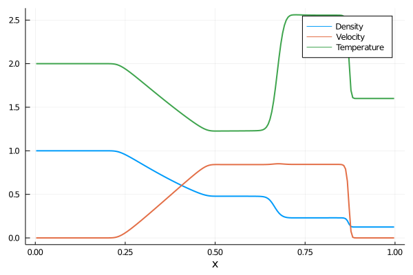
endThe result can be visualized with built-in function plot_line, which presents the profiles of gas density, velocity and temperature inside the tube.
plot_line(set, ctr)