Universal Boltzmann equation
In the following, we present a universal differential equation strategy to construct the neural network enhanced Boltzmann equation. The complicated fivefold integral operator is replaced by a combination of relaxation and neural models. It promises a completely differential structure and thus the neural ODE type training and computing becomes possible. The approach reduces the computational cost up to three orders of magnitude and preserves the perfect accuracy. The detailed theory and implementation can be found in Tianbai Xiao & Martin Frank, Using neural networks to accelerate the solution of the Boltzmann equation.
First we load all the packages needed and set up the configurations.
using Flux, Kinetic, OrdinaryDiffEq, Plots, SciMLSensitivity, Solaris

begin
    t1 = 3
    nt = 16
    u0 = -5
    u1 = 5
    nu = 80
    v0 = -5
    v1 = 5
    nv = 28
    w0 = -5
    w1 = 5
    nw = 28
    knudsen = 1
    inK = 0
    alpha = 1.0
    omega = 0.5
    nh = 8
end
The dataset is produced by the fast spectral method, which solves the nonlinear Boltzmann integral with fast Fourier transformation.
begin
    tspan = (0.0, t1)
    tsteps = linspace(tspan[1], tspan[2], nt)
    γ = heat_capacity_ratio(inK, 3)
    vs = VSpace3D(u0, u1, nu, v0, v1, nv, w0, w1, nw)

    f0 = @. 0.5 * (1 / π)^1.5 *
            (exp(-(vs.u - 1) ^ 2) + exp(-(vs.u + 1) ^ 2)) *
            exp(-vs.v ^ 2) * exp(-vs.w ^ 2)
    prim0 =
        conserve_prim(moments_conserve(f0, vs.u, vs.v, vs.w, vs.weights), γ)
    M0 = maxwellian(vs.u, vs.v, vs.w, prim0)
    mu_ref = ref_vhs_vis(knudsen, alpha, omega)
    τ0 = mu_ref * 2.0 * prim0[end]^(0.5) / prim0[1]

    # Boltzmann
    prob = ODEProblem(boltzmann_ode!, f0, tspan, fsm_kernel(vs, mu_ref))
    data_boltz = solve(prob, Tsit5(), saveat = tsteps) |> Array

    # BGK
    prob1 = ODEProblem(bgk_ode!, f0, tspan, [M0, τ0])
    data_bgk = solve(prob1, Tsit5(), saveat = tsteps) |> Array

    data_boltz_1D = zeros(Float64, axes(data_boltz, 1), axes(data_boltz, 4))
    data_bgk_1D = zeros(Float64, axes(data_bgk, 1), axes(data_bgk, 4))
    for j in axes(data_boltz_1D, 2)
        data_boltz_1D[:, j] .=
            reduce_distribution(data_boltz[:, :, :, j], vs.weights[1, :, :])
        data_bgk_1D[:, j] .=
            reduce_distribution(data_bgk[:, :, :, j], vs.weights[1, :, :])
    end
    f0_1D = reduce_distribution(f0, vs.weights[1, :, :])
    M0_1D = reduce_distribution(M0, vs.weights[1, :, :])

    X = Array{Float64}(undef, vs.nu, 1)
    for i in axes(X, 2)
        X[:, i] .= f0_1D
    end
    Y = Array{Float64}(undef, vs.nu, 1, nt)
    for i in axes(Y, 2)
        Y[:, i, :] .= data_boltz_1D
    end
    M = Array{Float64}(undef, nu, size(X, 2))
    for i in axes(M, 2)
        M[:, i] .= M0_1D
    end
    τ = Array{Float64}(undef, 1, size(X, 2))
    for i in axes(τ, 2)
        τ[1, i] = τ0
    end
end
Then we define the neural network and construct the unified model with mechanical and neural parts. The training is conducted by Solaris.jl with the Adam optimizer.
begin
model_univ = FnChain(
FnDense(nu, nu * nh, tanh),
FnDense(nu * nh, nu),
)
p_model = init_params(model_univ)
function dfdt(df, f, p, t)
df .= (M .- f) ./ τ .+ model_univ(M .- f, p)
end
prob_ube = ODEProblem(dfdt, X, tspan, p_model)
function loss(p)
sol_ube = solve(prob_ube, Midpoint(), u0 = X, p = p, saveat = tsteps)
loss = sum(abs2, Array(sol_ube) .- Y)
return loss
end
his = []
cb = function (p, l)
display(l)
push!(his, l)
return false
end
end
res = sci_train(loss, p_model, Adam(); cb = cb, maxiters = 200)
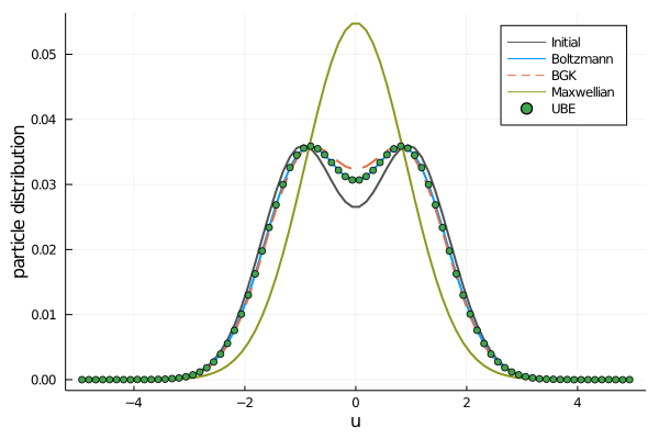
res = sci_train(loss, res.u, Adam(); cb = cb, maxiters = 200)Once we have trained a hybrid Boltzmann collision term, we could solve it as a normal differential equation with any desirable solvers. Consider the Midpoint rule as an example, the solution algorithm and visualization can be organized.
ube = ODEProblem(ube_dfdt, f0_1D, tspan, [M0_1D, τ0, (model_univ, res.u)])
sol = solve(
    ube,
    Midpoint(),
    u0 = f0_1D,
    p = [M0_1D, τ0, (model_univ, res.u)],
    saveat = tsteps,
)

plot(
    vs.u[:, vs.nv÷2, vs.nw÷2],
    data_boltz_1D[:, 1],
    lw = 2,
    label = "Initial",
    color = :gray32,
    xlabel = "u",
    ylabel = "particle distribution",
)
plot!(
    vs.u[:, vs.nv÷2, vs.nw÷2],
    data_boltz_1D[:, 2],
    lw = 2,
    label = "Boltzmann",
    color = 1,
)
plot!(
    vs.u[:, vs.nv÷2, vs.nw÷2],
    data_bgk_1D[:, 2],
    lw = 2,
    line = :dash,
    label = "BGK",
    color = 2,
)
plot!(
    vs.u[:, vs.nv÷2, vs.nw÷2],
    M0_1D,
    lw = 2,
    label = "Maxwellian",
    color = 10,
)
scatter!(vs.u[:, vs.nv÷2, vs.nw÷2], sol.u[2], lw = 2, label = "UBE", color = 3)